mlforecast

Machine Learning 🤖 Forecast
Scalable machine learning for time series forecasting
![]()


mlforecast is a framework to perform time series forecasting using machine learning models, with the option to scale to massive amounts of data using remote clusters.
Install
PyPI
pip install mlforecast
conda-forge
conda install -c conda-forge mlforecast
For more detailed instructions you can refer to the installation page.
Quick Start
Minimal Example
import lightgbm as lgb

from mlforecast import MLForecast
from sklearn.linear_model import LinearRegression

mlf = MLForecast(
    models = [LinearRegression(), lgb.LGBMRegressor()],
    lags=[1, 12],
    freq = 'M'
)
mlf.fit(df)
mlf.predict(12)
Get Started with this quick guide.
Follow this end-to-end walkthrough for best practices.
Sample notebooks
Why?
Current Python alternatives for machine learning models are slow,
inaccurate and don’t scale well. So we created a library that can be
used to forecast in production environments. MLForecast includes
efficient feature engineering to train any machine learning model (with
fit and predict methods such as
sklearn) to fit millions of time
series.
Features
- Fastest implementations of feature engineering for time series forecasting in Python.
- Out-of-the-box compatibility with Spark, Dask, and Ray.
- Probabilistic Forecasting with Conformal Prediction.
- Support for exogenous variables and static covariates.
- Familiar
sklearnsyntax:.fitand.predict.
Missing something? Please open an issue or write us in
Examples and Guides
📚 End to End Walkthrough: model training, evaluation and selection for multiple time series.
🔎 Probabilistic Forecasting: use Conformal Prediction to produce prediciton intervals.
👩🔬 Cross Validation: robust model’s performance evaluation.
🔌 Predict Demand Peaks: electricity load forecasting for detecting daily peaks and reducing electric bills.
📈 Transfer Learning: pretrain a model using a set of time series and then predict another one using that pretrained model.
🌡️ Distributed Training: use a Dask, Ray or Spark cluster to train models at scale.
How to use
The following provides a very basic overview, for a more detailed description see the documentation.
Data setup
Store your time series in a pandas dataframe in long format, that is, each row represents an observation for a specific serie and timestamp.
from mlforecast.utils import generate_daily_series

series = generate_daily_series(
    n_series=20,
    max_length=100,
    n_static_features=1,
    static_as_categorical=False,
    with_trend=True
)
series.head()| unique_id | ds | y | static_0 | |
|---|---|---|---|---|
| 0 | id_00 | 2000-01-01 | 17.519167 | 72 |
| 1 | id_00 | 2000-01-02 | 87.799695 | 72 |
| 2 | id_00 | 2000-01-03 | 177.442975 | 72 |
| 3 | id_00 | 2000-01-04 | 232.704110 | 72 |
| 4 | id_00 | 2000-01-05 | 317.510474 | 72 |
Models
Next define your models. If you want to use the local interface this can
be any regressor that follows the scikit-learn API. For distributed
training there are LGBMForecast and XGBForecast.
import lightgbm as lgb
import xgboost as xgb
from sklearn.ensemble import RandomForestRegressor

models = [
    lgb.LGBMRegressor(verbosity=-1),
    xgb.XGBRegressor(),
    RandomForestRegressor(random_state=0),
]
Forecast object
Now instantiate a MLForecast object with the models and the features
that you want to use. The features can be lags, transformations on the
lags and date features. The lag transformations are defined as
numba jitted functions that transform an
array, if they have additional arguments you can either supply a tuple
(transform_func, arg1, arg2, …) or define new functions fixing the
arguments. You can also define differences to apply to the series before
fitting that will be restored when predicting.
from mlforecast import MLForecast
from mlforecast.target_transforms import Differences
from numba import njit
from window_ops.expanding import expanding_mean
from window_ops.rolling import rolling_mean


@njit
def rolling_mean_28(x):
    return rolling_mean(x, window_size=28)


fcst = MLForecast(
    models=models,
    freq='D',
    lags=[7, 14],
    lag_transforms={
        1: [expanding_mean],
        7: [rolling_mean_28]
    },
    date_features=['dayofweek'],
    target_transforms=[Differences([1])],
)
Training
To compute the features and train the models call fit on your
Forecast object.
fcst.fit(series)MLForecast(models=[LGBMRegressor, XGBRegressor, RandomForestRegressor], freq=<Day>, lag_features=['lag7', 'lag14', 'expanding_mean_lag1', 'rolling_mean_28_lag7'], date_features=['dayofweek'], num_threads=1)
Predicting
To get the forecasts for the next n days call predict(n) on the
forecast object. This will automatically handle the updates required by
the features using a recursive strategy.
predictions = fcst.predict(14)
predictions| unique_id | ds | LGBMRegressor | XGBRegressor | RandomForestRegressor | |
|---|---|---|---|---|---|
| 0 | id_00 | 2000-04-04 | 299.923771 | 309.664124 | 298.424164 |
| 1 | id_00 | 2000-04-05 | 365.424147 | 382.150085 | 365.816014 |
| 2 | id_00 | 2000-04-06 | 432.562441 | 453.373779 | 436.360620 |
| 3 | id_00 | 2000-04-07 | 495.628000 | 527.965149 | 503.670100 |
| 4 | id_00 | 2000-04-08 | 60.786223 | 75.762299 | 62.176080 |
| ... | ... | ... | ... | ... | ... |
| 275 | id_19 | 2000-03-23 | 36.266780 | 29.889120 | 34.799780 |
| 276 | id_19 | 2000-03-24 | 44.370984 | 34.968884 | 39.920982 |
| 277 | id_19 | 2000-03-25 | 50.746222 | 39.970238 | 46.196266 |
| 278 | id_19 | 2000-03-26 | 58.906524 | 45.125305 | 51.653060 |
| 279 | id_19 | 2000-03-27 | 63.073949 | 50.682716 | 56.845384 |
280 rows × 5 columns
Visualize results
from utilsforecast.plotting import plot_seriesfig = plot_series(series, predictions, max_ids=4, plot_random=False)
fig.savefig('figs/index.png', bbox_inches='tight')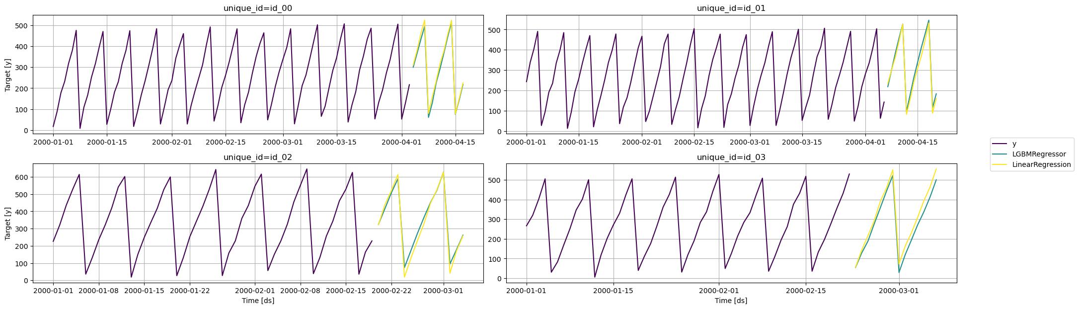
How to contribute
See CONTRIBUTING.md.